Satellite images object detection – Part 2: the beauty & the beast
Part two of a three-part series looking into ship surveillance and tracking with satellite imaging.
Ship surveillance & tracking – part 2: towards fully convolutional network, for more interpretability (example of CAM attention), early localisation properties, and capability to evolve into an image segmentation model. In the process, we’ll delve into the technique of transfer learning.
Motivation: although the simple ConvNet we built in Part 1 did pretty well at the classification task we gave it, the usage of dense layers makes it hard to interpret, both by human, and for further models to be built on top of it. In this post, we explore a different ConvNet structure that uses convolutional layers and pooling layers instead of dense layers, keeping connections localised. It is not only more interpretable when used for classification, but can also evolve into an object localisation / segmentation model, which we will present in part 3, with a U-Net.
While we’d like to start with the beauty, we often need to face the beast first:
- The beast: insights into some of the unspoken practical challenges with transfer learning
- The beauty: decision interpretability through GAP/GMP’s pooling implicit localisation properties
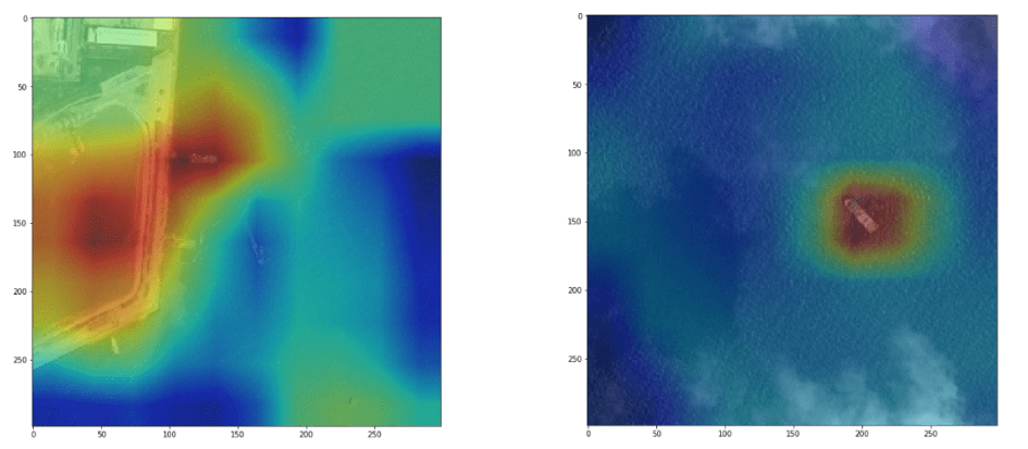
Visualisation of the model’s attention, and with it emerging localisation properties. More details at the end of this post.
This is the 2nd part of a 3 blog posts series:
- Ship detection – Part 1: binary prediction of whether there is at least 1 ship, or not. Part 1 is a simple solution showing great results in a few lines of code
- Ship detection & early localisation- Part 2: towards object segmentation with (a) training fully convolutional NN through transfer learning, to build an encoder for a U-Net, and (b) first emerging localisation properties with CAM attention interpretability
- Ship localisation – Part 3: identify where ships are within the image, building a U-Net from the encoder developed in Part 2
What you will learn in this post (Ship detection – Part 2):
- Encoder for a U-Net: training a fully convolutional network on a classification task
- Transfer learning: a brief review of the image recognition architectures
- Practical transfer learning from MobileNetV2 and Xception, reaching 93% accuracy after having seen only 0.5 times the data set, along with the practical challenges involved in using and fine-tuning those complex pre-trained networks.
- Learning rate tuning techniques, such as landscaping and cycling to get out of local optima
- Visualise model attention and implicit localisation through the interpretation of hidden layers when Global Average / Max Pooling is used (GAP / GMP). In contrast to classic localisation algorithms that use localisation labels for training, this network remarkably learns basic localisation implicitely, with only ship / no ship labels
Transfer learning from pre-trained deep ConvNets
Transfer learning is the idea that strong neural networks trained for one application have generalisable features that can be leveraged for other applications. This means a large network fine-tuned for weeks on problems such as ImageNet, with 1000 classes and 1.2 million images, would have learned something fundamental about processing features, e.g. detecting edges, managing contrasts, etc.
To take advantage of such models, the first step is to use the pre-trained model as a feature extractor and add a simple classifier on top, and if performance and the data set warrants it, fine tune some layers of the pre-trained model.
Training those networks is expensive though: for example with ResNet50V2 the iteration time on my machine (CPU only) was 12h per pseudo-epoch vs 35min for the simple ConvNet presented in Part 1 (side note: with GPU you get a 15x increase in speed so that changes the game).
To choose what network to transfer from, I took a look at the performance on the ImageNet competition. A word on popular networks you may want to use for transfer learning:
- Residual Nets: although deeper neural networks tend to make better use of neurons than wide shallow networks, they suffer from vanishing gradients, as the back propagation feedback from the loss function gets passed from layer to layer. ResNets tackled this problem by creating shortcuts that facilitate this backwards information transfer, and effectively make it very easy for each module to learn the identity function instead of bad performance that’d harm other layers. Note those shortcuts are “short skips” on a ResNet, and we’ll explore “long skips” with U-nets in the next blog post on localisation (Part 3).
- Inception Nets: core idea is to enable filters of multiple sizes to operate at the same level in the network, and let the network chose which is best placed to pick the right feature, depending e.g. on the size of the object on the image. To keep computational cost under control, a 1×1 depth filter is introduced to reduce the number of channel (effectively creating a bottleneck). More than InceptionV3, one of the most successful network with this architecture seems to be Xception.
- MobileNet: ResNet trying to be more light weight by performing depth-wise convolutions (to reduce the number of channels), and use bottleneck layers (a bit like InceptionNet is seems). The goal here is to keep high performance in environments with limited compute, such as mobile phones.
First go at transfer learning on TensorFlow 2.0 with MobileNetV2
Given my computer’s performance limitations, I had a go at MobileNetV2, and got a pseudo-epoch iteration time of 2.5h (CPU).
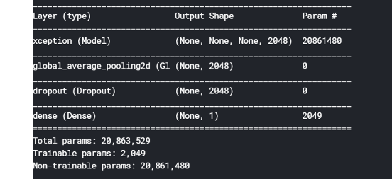
Using the pretrained model as a feature extractor, a classifier can be built by adding 2 layers:
- a global pooling layer to aggregate the features over the spatial dimensions: (batch size, height, width, channels) -> (batch size, 1, 1, channels), irrespective of image size. I chose global max pooling instead of global average pooling as I have the intuition average pooling would favour larger ship on the image.
- adding a simple neuron to interpret those features as a sign of a vessel vs not. Basically, this is equivalent to building logistic regression on top of 1280 features.
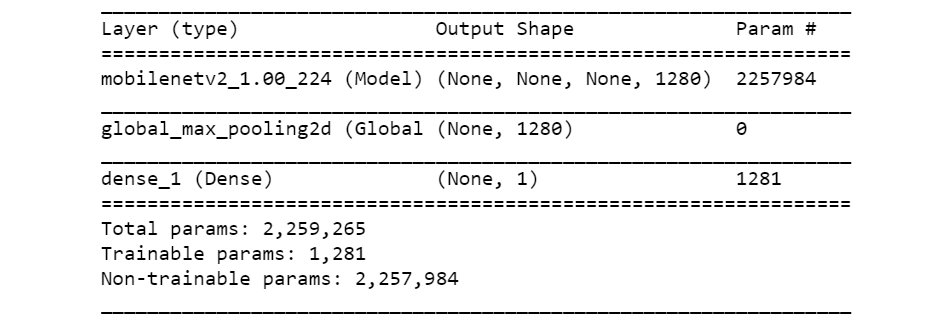
The model quickly converged to 77.5% accuracy, which may sound ok, but actually corresponds to the class imbalance. Looking more closely, the model only learned to always predict “no ship”, and the loss stayed flat for 5 pseudo-epochs (i.e. over 200k images). I explored a range of learning rates, but this didn’t change much:
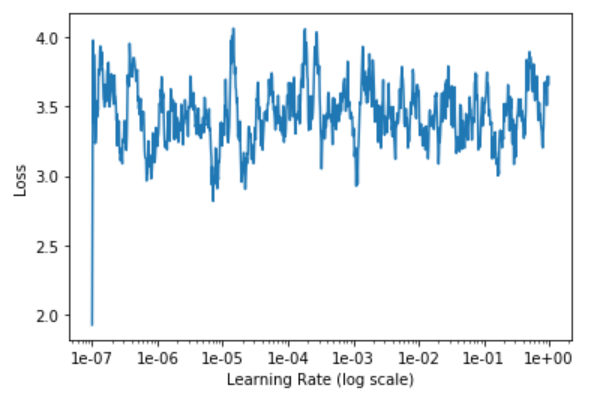
Although the model may not have enough capacity, and acknowledging the ImageNet dataset is pretty different from our satellite images of ship, I felt such a bad performance was suspicious.
I tried feeding the network repeatedly the same single batch of 40 images to see if the model is able to fully overfit, but it didn’t seem to? The model clearly has enough capacity to learn by heart 40 results.
Turns out there was an error in the TF documentation, as raised in this Github issue: binary_crossentropy expects by default a probability, not a logit (raw value, without activation). Fix in flight
Lessons learned: trying to overfit a single batch to check the feedback mechanism works can be a pretty handy sanity check tool
Second go at transfer learning on TensorFlow 2.0 with MobileNetV2
Training single neuron dense layer (only 1k parameters).
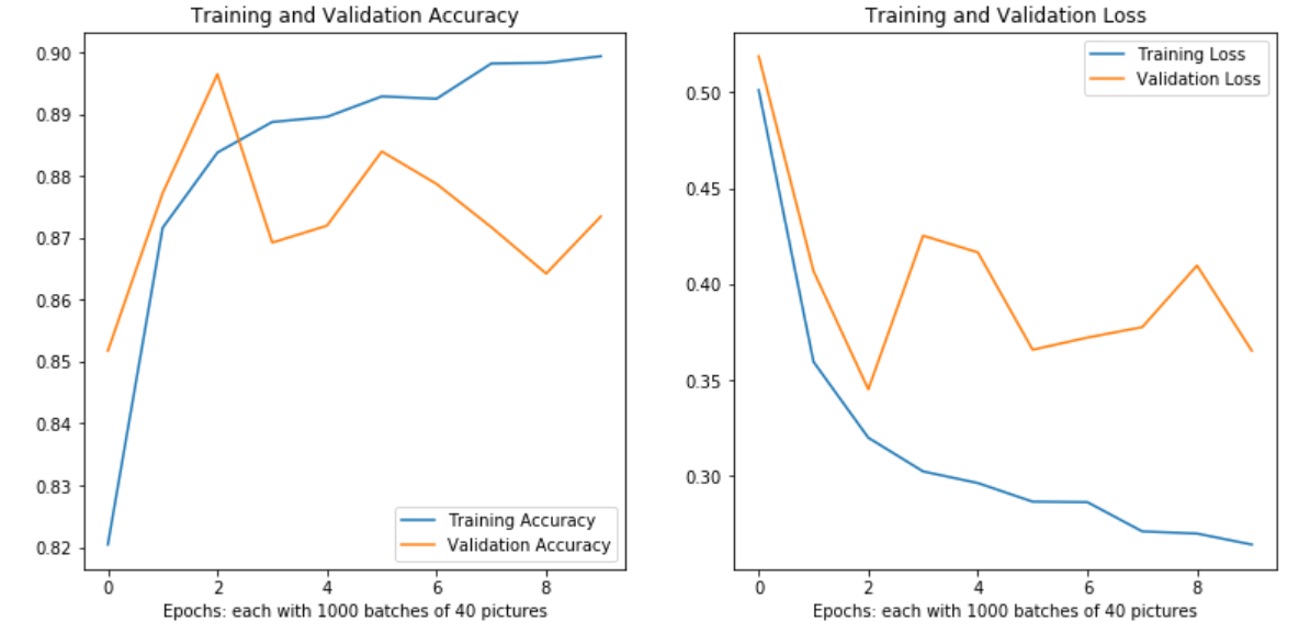
With transfer learning we observe quickly very high performance while only training 1k parameters. However, strangely the model starts to overfit despite so few parameters.
I tried adding dropouts, and even 50% didn’t curb the model’s overfit. I tried GAP instead of GMP to spatially regularise, and performance went down closer to 80% than 90%. The ImageNet images are pretty different from ours, so I decided to fine tune the last layers of the network with a small learning rate (3E-5), and got a boost in performance initially, and very quickly more overfitting. I didn’t try increasing the training set size as the model starts overfitting before having seen the entire data set!
At this point I thought the model may be stuck on a local optima, may benefit from larger images, fine tuning of deeper layers, or counter intuitively need more capacity / a new architecture. Let’s try some of those!
Transfer learning from Xception network, and learning rate cycling to get out of local optima
We first get a baseline with Xception of training the base classifier + fine tuning, without learning rate cycling:
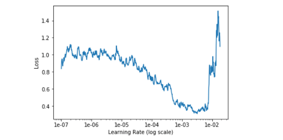
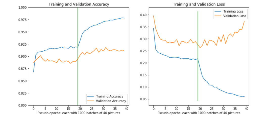
You can observe that fine tuning initially gives a boost in CV accuracy, but leads to aggressive overfitting.
Now we explore learning rate cycling to speed up learning and hopefully escape local optimum (code):
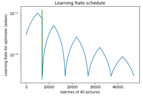
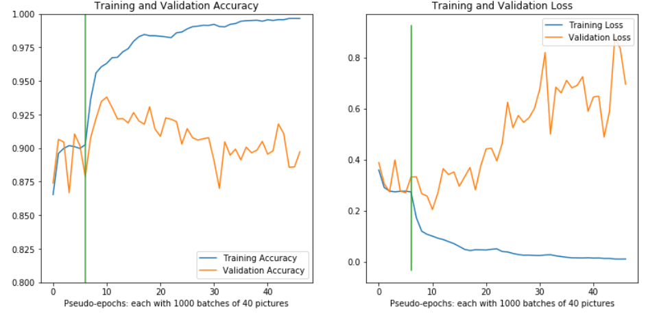
Learning rate cycling speeds up training, and gives a CV accuracy boost, but does not solve the underlying overfitting problem.
Best result is achieved with early stopping at about 12 epochs. We decided to stop fine tuning for this post: further improvements could explore:
- using progressively larger images: this can be changed in the argument of our pipeline ImageBatchGenerator, since we left the input size of our Xception model as None, and the GAP/GMP layer makes the classifier size-invariant.
- train for longer, with an augmented data set (distortions, more images etc)
- further regularisation
Conclusion with transfer learning: although this can give great results fast on problems similar to the pretraining dataset, miracles shouldn’t be expected and quite a bit of work is needed in practice to extract the last percentages of accuracy. As we saw in this post, simpler solutions should not be overlooked!
That being said, we’ve got a pretty decent classifier with 94% accuracy, and that will be enough as a basis for our U-Net in Part 3.
Now we will look into a cool feature of networks using GAP / GMP layers: interpretability of hidden layers and localisation as an emerging behaviour.
The concept of network’s attention, and with it implicitly learned object localisation
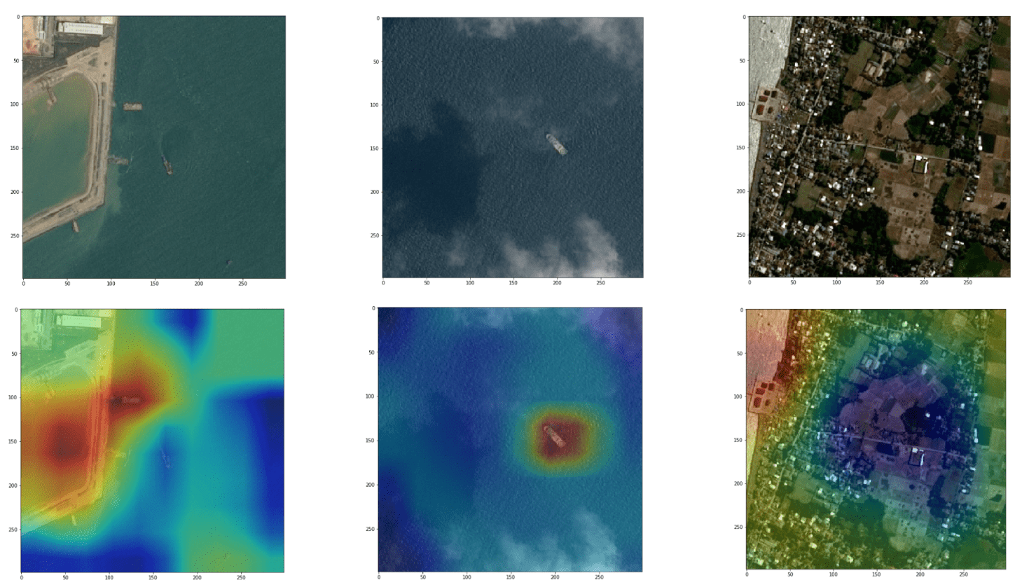
Neural networks have a reputation for being hard to interpret, and are often described as black boxes. With CNNs using global pooling layers, an activation map indicating the discriminative image regions used by the network can easily be calculated.
Just before the final output layer, we have performed global pooling on the convolutional feature maps, and then used those features in a fully-connected layer producing the desired classification. Given this simple connectivity structure, we can identify the importance of the image regions by projecting back the weights of the output layer on to the convolutional feature maps, a technique known as Class Activation Mapping (CAM).
Another way to understand this is to look at our simplified architecture:
- Image inputs: (batch size=40, height=299, width=299, channels=3)
- Xception output: (batch size=40, height at this layer=10, width at this layer=10, channels at this layer=2048)
- Global Max Pooling output: (batch size=40, 1, 1, channels at this layer=2048)
- Classifier (dense) output: (batch size=40, classification dim=1)
The quantity we show on the heatmap is the Xception output, summed over the channels axis, with the sum weighted by the Classifier’s weights for each channel.
This simple quantity can be directly visualised. In practice though the resolution is quite low (10×10), as we are deep into the network , so in the visualisation above we have upsampled it (back to 299×299 to overlay with original image).
Core part of the calculation. The dotprod is what we show on the heatmap, after upsampling. More detailed example here.
I hope you enjoyed the ride and got some good takeaway. I’d love to hear of your own experience with transfer learning, and whether there are steps in the analysis you interpret differently! In the next post, we will reuse the Xception classifier we trained in this post to 94% accuracy, and will reuse it as the encoder of our U-Net for image segmentation / ship localisation.